Electric field of a uniformly charged plate. Application of Gauss's theorem to calculate the field of an infinite uniformly charged plane

Let us find the distribution of the field potential created by two identical uniformly charged parallel plates, the charges of which are equal in magnitude and opposite in sign 1 (Fig. 279).

Rice. 279
Let us denote the surface charge density on one plate +σ , and on the other −σ . Distance between plates h we will assume that it is significantly smaller than the size of the plates. Let us introduce a coordinate system, axis z which is perpendicular to the plates, the origin of coordinates will be placed in the middle between the plates. Obviously, for infinitely large plates, all field characteristics (strength and potential) depend only on the coordinate z. To calculate the field strength at various points in space, we will use the resulting expression for the field strength created by an infinite uniformly charged plate and the superposition principle.
Each uniformly charged plate creates a uniform field, the modulus of which is equal to E o = σ/(2ε o), and the directions are indicated in Figure 280, 281.



rice. 280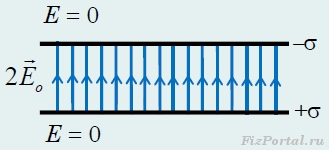

rice. 281
Adding the field strengths according to the superposition principle, we obtain that in the space between the plates the field strength E = 2E o = σ/ε o twice the field strength of one plate (here the fields of the individual plates are parallel), and there is no field outside the plates (here the fields of the individual plates are opposite).
Strictly speaking, for plates of finite sizes the field is not uniform; the field lines of the plates of finite sizes are shown in Figure 282.



rice. 282
The strongest deviations from homogeneity are observed near the edges of the plates (often these deviations are called edge effects). However, in the region adjacent to the middle of the plates the field can be considered homogeneous with a high degree of accuracy, that is, in this region edge effects can be neglected. Note that the smaller the ratio of the distance between the plates to their sizes, the smaller the errors in this approximation.
To unambiguously determine the distribution of the field potential, it is necessary to select the level of zero potential. We will assume that the potential is equal to zero in the plane located in the middle between the plates, that is, we put φ = 0 at z = 0.
Despite the arbitrariness in choosing the zero potential level, our choice can be logically justified based on the symmetry of the system. Indeed, the system of charges under consideration repeats itself in mirror reflection relative to the plane z = 0 and a simultaneous change in the signs of the charges. Therefore, it is desirable that the potential distribution have the same symmetry: it is restored upon mirror reflection with a simultaneous change in the sign of all field functions. The method we have chosen for selecting the zero potential satisfies this symmetry.



rice. 283
Let us denote the potential of a positively charged plate +φ o, then the potential of the negatively charged plate will be equal to φo. These potentials can be easily determined using the found value of the field strength between the plates and the relationship between the strength and the potential difference electric field. The equation of this connection in this case has the form +φo − φ o = Eh. From this relationship we determine the values ​​of the plate potentials φ o = σh/(2ε o). Considering that the field is uniform between the plates (therefore the potential changes linearly), and there is no field outside the plates (therefore the potential is constant here), the dependence of the potential on the coordinate z looks like (Fig. 284)

rice. 284

 Assignments for independent work.
 1. In all the examples considered, perform the reverse operation: using the found potential distribution using the formula E x = −Δφ/Δx calculate the strengths of the considered fields.
 2. Derive formula (6) strictly.
 3. Qualitatively explain the following “paradox”. In the field of a flat capacitor, the “infinity” potential is ambiguously defined: when moving in the positive direction of the axis Z the potential of “infinity” turned out to be equal −φ o; when moving in a negative axis direction Z − +φ o, when moving along the axes X or Y− is equal to zero. So what is the potential of “infinity” in a real system of two plates of finite sizes?

1 Such a system is called flat capacitor, we will study these devices in more detail later.

Previously we showed that electric field, created by an infinite uniformly charged plate is homogeneous, that is, the field strength is the same at all points, and the intensity vector is directed perpendicular to the plane, and its modulus is equal to E o = σ/(2ε o). The family of force lines of such a field is a set of parallel lines perpendicular to the plate. In Fig. 275, 276 also shows a graph of the projection of the field strength vector E z per axis Z perpendicular to the plate (we will place the origin of this axis on the plate). It is clear that the potential of this field depends only on the coordinate z, that is, the equipotential surfaces in this case are planes parallel to the charged plate.



rice. 275



rice. 276
With the traditional choice of zero potential level φ(z → ∞), the potential of an arbitrary point is equal to the work of moving a unit positive charge from a given point to infinity. Since the modulus of tension is constant, such work (and, consequently, potential) turns out to be equal to infinity! Consequently, the specified choice of zero potential level is unsuitable in this case.
Therefore, you should take advantage of the arbitrariness of choosing the zero level. It is enough to select an arbitrary point with coordinate z = z o, and assign to it an arbitrary potential value φ(z o) = φ o(Fig. 277).

rice. 277
Now, to calculate the potential value at an arbitrary point φ(z), you can use the relationship between field strength and potential

Considering that in this case the field strength is constant (at z > 0) this expression is written in the form

from which follows the desired dependence of the potential on the coordinate (at z > 0)

In particular, you can set an arbitrary value of the potential of the plate itself, that is, set at z = z o = 0, φ = φ o. Then the value of the potential at an arbitrary point is determined by the function

the graph of which is shown in Figure 278.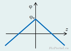

rice. 278
The fact that the potential relative to infinity turned out to be infinitely large is quite obvious - after all, an infinite plate also has an infinitely large charge. As we have already emphasized, such a system is an idealization - infinite plates do not exist. In reality, all bodies have finite dimensions, so for them the traditional choice of zero potential is possible, although in this case the field distribution can be very complex. Within the framework of the idealization under consideration, it is more convenient to use the choice of the zero level that we used.

Let's assume the charge is positive. The plane is charged with a constant surface density. From symmetry it follows that the intensity at any point of the field has a direction perpendicular to the plane (Fig. 2.10). It is obvious that at points symmetrical relative to the plane, the field strength is the same in magnitude and opposite in direction.

Let us select an area on the charged plane. Let's surround this area with a closed surface. As a closed surface, let us imagine a cylindrical surface with generatrices perpendicular to the plane and bases of magnitude , located symmetrically relative to the plane. Let us apply Gauss's theorem to this surface . There will be no flow through the side of the surface, since at each point it is zero. For bases the same as . Therefore, the total flux through the surface will be equal to . There is a charge inside the surface. According to Gauss's theorem, the following condition must be satisfied: , where . (3)

The result obtained does not depend on the length of the cylinder, i.e. at any distance from the plane the field strength is the same in magnitude. The picture of tension lines looks as shown in Fig. 2.11. For a negatively charged plane, the directions of the vectors will change to the opposite. If the plane is of finite dimensions, then the result obtained will be valid only for points whose distance from the edge of the plate significantly exceeds the distance from the plate itself (Fig. 2.12).