Electrical circuits are complex so better. Complex DC electrical circuits
5. Basic methods of analysis of linear electrical circuits.
greatly simplifies the calculation loop current method, since it reduces the number of equations.
When calculating by this method, it is assumed that each independent circuit of the circuit has its own circuit current. The equations are made with respect to the loop currents, after which the branch currents are determined through them.
overlay method: the current in any branch is equal to the algebraic sum of the currents caused by each of the E.D.S. schemes separately. Linear electrical circuit is described by the system linear equations Kirchhoff. This means that it obeys the principle of superposition (superposition), according to which the combined action of all sources in the electrical circuit coincides with the sum of the actions of each of them separately.
A method for calculating electrical circuits, in which the potentials of the circuit nodes are taken as unknowns, called the method of nodal potentials. The number of unknowns in the method of nodal potentials is equal to the number of equations that must be compiled for the circuit according to Kirchhoff's I law. The method of nodal potentials, like the method of loop currents, is one of the main calculation methods. In the case when p-1< p (n – количество узлов, p – количество независимых контуров), данный метод более экономичен, чем метод контурных токов.
6. Causes and essence transients.
The transition from one stationary state to another does not occur instantly, but over time, due to the presence of energy storage devices (inductances of coils and capacitances of capacitors) in the circuit. The magnetic energy of the coils and Electric Energy capacitors cannot change abruptly, because To accomplish this, sources of infinite power are needed. The processes that accompany this transition are called transitional.
7. Analysis of transient processes in the time domain. Classic method
The classical method for calculating transients is based on the compilation and subsequent solution (integration) of differential equations compiled according to Kirchhoff's laws and relating the desired currents and voltages of the post-switching circuit and the given influencing functions (sources of electrical energy. By transforming the system of equations, one can derive the final differential equation with respect to some either one variable x(t):
Here n – order differential equation, which is also the order of the chain, the coefficients a k> 0 and are determined by the parameters of passive elements R,L,C chain, and the right side is a function of the setting actions.
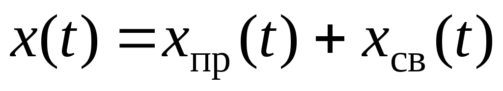
In accordance with the classical theory of differential equations, the complete solution of an inhomogeneous differential equation is found as the sum of a particular solution of an inhomogeneous differential equation and a general solution of a homogeneous differential equation:
H 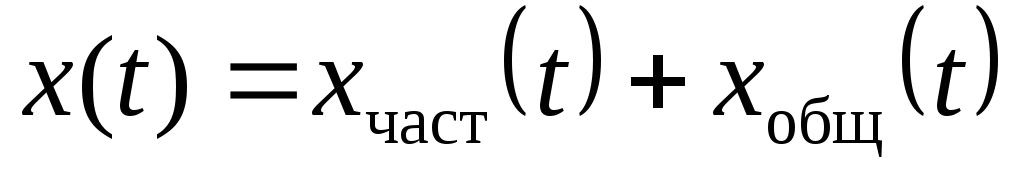 The actual solution is completely determined by the form of the right-hand side f(t) differential equation. In electrical problems, the right side depends on the influencing sources of electrical energy, so the form
 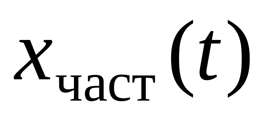 is conditioned (forced) by sources of electrical energy and is called forced component.
The general solution of a homogeneous differential equation depends on the roots characteristic equation, which are determined by the coefficients of the differential equation, and does not depend on the right side. Thus, any desired value in the transition mode
 .
.
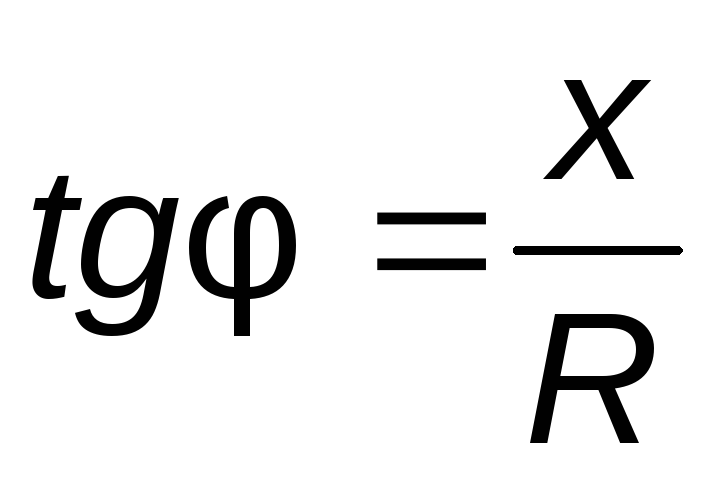
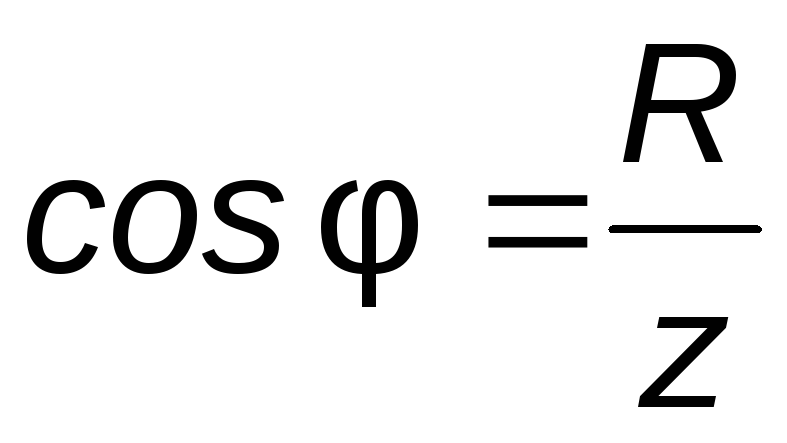
16. Active reactive and impedance. Resistance Triangle
 .
.
From this it follows that the modulus of complex resistance:
 .
(3.44)
.
(3.44)
WITH 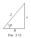 Therefore, z can be represented as the hypotenuse of a right-angled triangle (Fig. 3.13) - a triangle of resistances, one leg of which is equal to R, the other is x.
Wherein
 ,
(3.45)
,
(3.45)
 .
(3.46)
.
(3.46)
Knowing  or
or 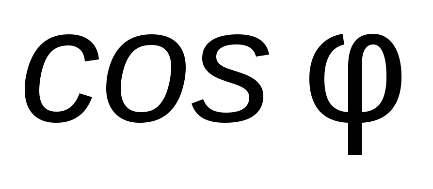 , you can define the angle
  .
.
Angle sign in expressions for the instantaneous value of the current  determined by the nature of the load: with an inductive nature of the load (
  ) the current lags the voltage by an angle and in the expression for the instantaneous value of the current, the angle written with a minus sign, that is; with capacitive load (
 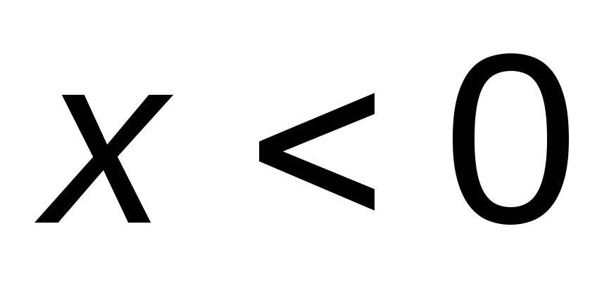 ) the current leads the voltage by an angle and the expression for the instantaneous value of the current is written with a plus sign, that is.
17. Stress resonance. Coeff. Power. Power Triangle.
Corresponds to the case when  (Fig. 3.16). Wherein
 ![]() (see section 3.10 for details).
(see section 3.10 for details).
From formula 3.41, we can conclude that the powers P, Q, S are related by the following relationship:
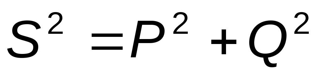 .
(3.47)
.
(3.47)
G 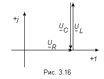
 This relationship can be represented graphically as right triangle(Fig. 3.17) - a triangle of power, which has a leg equal to P, a leg equal to Q and a hypotenuse S.
The ratio of P to S, equal to , is called power factor.
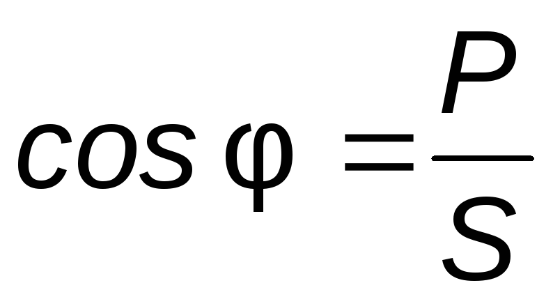 .
(3.48)
.
(3.48)
In practice, one always strives to increase , since reactive power, which always exists in the circuit R, L, C, is not consumed, but only active is used. From this we can conclude that reactive power is superfluous and unnecessary.
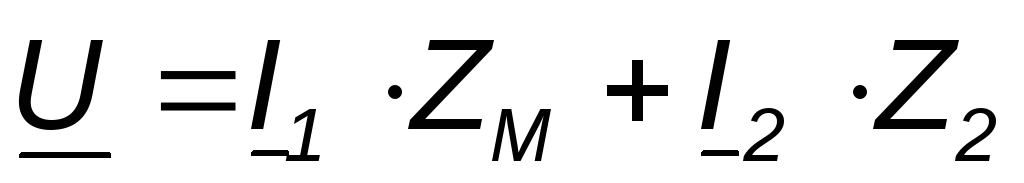
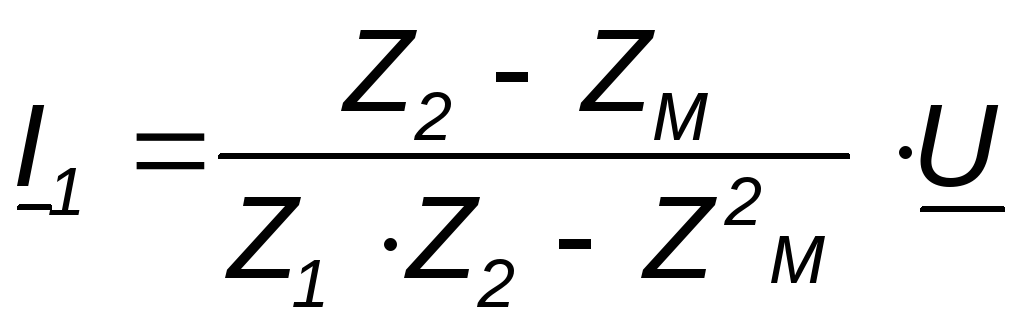
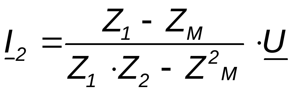
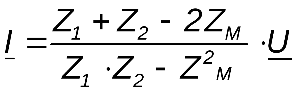
21. Parallel connection of inductively coupled circuit elements
![]()
Two coils with resistances R 1 and R 2, inductances L 1 and L 2 and mutual inductance M are connected in parallel, and the conclusions of the same name are connected to the same node (Fig. 4.7).
With the chosen positive directions of currents and voltages, we obtain the following expressions:
 ;
(4.11)
;
(4.11)
 ;
(4.12)
;
(4.12)
 ;
(4.13)
;
(4.13)
Where  (4.14)
In these equations complex stresses
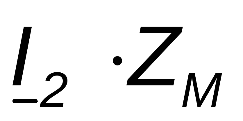 And
And 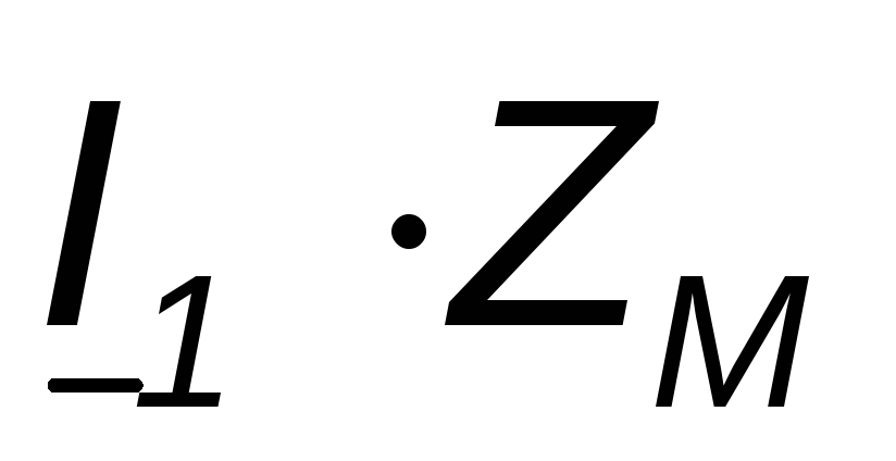 are taken with a plus sign, since the positive directions of these voltages (selected from top to bottom) and those currents on which these voltages depend are oriented in the same way relative to the same terminals. Solving the equations, we get
 ;
(4.15)
;
(4.15)
 ;
(4.16)
;
(4.16)
 .
(4.17)
.
(4.17)
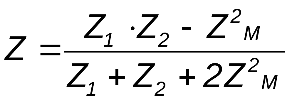
Whence it follows that the input complex resistance of the circuit under consideration
 .
(4.18)
.
(4.18)
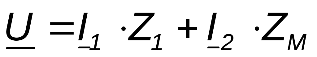
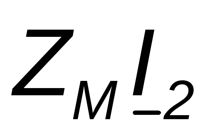
Let us now consider an inclusion in which like-named pins are connected to different nodes, i.e., L 1 and L 2 are connected to the node by different-named pins. In this case, the positive directions of the mutual induction voltages (selected from top to bottom) and those currents on which they depend are unequally oriented relative to the same terminals and the complex voltages  And
And
 will enter equations (4.12) and (4.13) with a minus sign. For currents
  expressions similar to (4.15-4.17) will be obtained, with the difference that Z M is replaced by -
Z M and the input impedance of the circuit
expressions similar to (4.15-4.17) will be obtained, with the difference that Z M is replaced by -
Z M and the input impedance of the circuit
 .
(4.19)
.
(4.19)
25. Definition of a quadripole. The main forms of writing the quadripole equations
In some cases it is necessary to consider electrical circuits with two input and two output terminals in which the input current and voltage are coupled linear dependencies with voltage and current output.
Such chains are called quadripoles. They can have an arbitrarily complex structure, since in the process of studying the circuit it is important to determine not the currents and voltages in individual branches, but only the dependencies between the input and output voltages and currents.
Sometimes called quadripoles electrical apparatus and devices having a pair of input and a pair of output terminals. These include, for example, single-phase transformers, power line sections, diode bridge rectifiers, smoothing filters, and so on.
The conditional image of a quadripole is shown in fig. 7.1.
ABOUT ![]() bottom pair of conclusions are called input (denoted
bottom pair of conclusions are called input (denoted  ), the other - days off (denoted
  ).
).
If a four-terminal network does not contain sources of electrical energy, then it is called passive, and if it contains - active.
An example of an active quadripole is an electronic amplifier.
In the diagram, an active four-pole is depicted as a rectangle with the letter A. A passive four-terminal is indicated by the letter P, or not indicated at all.
If both pairs of clamps are working for a quadripole, then it is called checkpoint.
A four-terminal network, in fact, is a transfer link between a power source and a load. To input terminals  , as a rule, connect the power supply, to the output terminals
  - load.
The relationships between two voltages and two currents at the input and output terminals can be written in various forms.
The following six forms of writing the passive four-terminal equations are possible:
Form A(main):
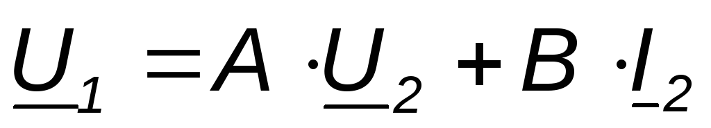 ,
(7.1)
,
(7.1)
 ,
(7.2)
,
(7.2)
where A,D are dimensionless coefficients;
C - [Cm] \u003d [Ohm -1]
27. Method of equivalent generator
IN  In practical calculations, it is often not necessary to know the operating modes of all elements of a complex circuit, but the task is to investigate the operating modes of one specific branch.
When calculating a complex electrical circuit, you have to perform significant computational work even when you want to determine the current in one branch. The volume of this work increases several times if it is necessary to establish a change in current, voltage, power when the resistance of a given branch changes, since calculations must be performed several times, setting different meanings resistance.
In any electrical circuit, one can mentally single out one branch, and the rest of the circuit, regardless of structure and complexity, can be conditionally depicted as a rectangle, which is the so-called two-terminal network.
Thus, a two-terminal network is a generalized name for a circuit that is connected to a selected branch with two output terminals (poles). If there is a source of E.D.S. in a two-terminal network. or current, then such a two-terminal network is called active. If there is no source of E.D.S. in a two-terminal network. or current, then it is called passive.
When solving the problem by the equivalent generator method (active two-terminal network), it is necessary:
1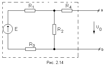 . Mentally conclude the entire circuit containing the E.D.S. and resistance, into a rectangle, selecting a branch from it ab, in which you want to find the current (Figure 2.13).
Find the voltage at the terminals of the open branch ab(at idle).
The open-circuit voltage Uo (equivalent to E.D.S. Ee) for the circuit under consideration can be found as follows:  .
.
The resistance R4 was not included in the calculation, since when the branch ab is open, the current does not flow through it.
3. Find the equivalent resistance. At the same time, the sources of E.D.S. are short-circuited, and the branches containing current sources are opened. The bipolar becomes passive.
D 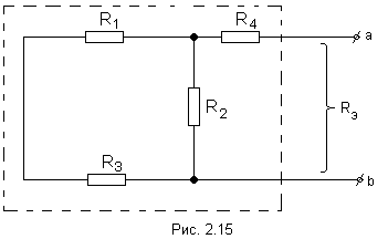 for this scheme
 .
.
4. Calculate the current value. For this scheme, we have:  .
.
In a complex electrical circuit direct current(Table 2)
determine the currents in all sections of the circuit. The problem can be solved by any two methods
table 2
| Option No. | Data for calculations | Electrical circuit diagram |
| E 1 \u003d 136V; E 2 \u003d 80V; R 1 \u003d 194 ohms; R 2 \u003d 76 ohms; R 3 \u003d 240 ohms; R 4 \u003d 120 ohms. . r 1 \u003d 6 ohms; r 2 \u003d 4 ohms. | Fig.12 | |
| E 1 \u003d 150V; E 2 \u003d 170V; R 1 \u003d 29.5 Ohm; R 2 \u003d 24 Ohm; R 3 \u003d 40 Ohm; r 1 \u003d 0.5 Ohm; r 2 \u003d 1 Ohm. | 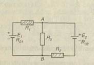 Fig.13 Fig.13 |
|
| E 1 \u003d 68V; E 2 \u003d 40V; R 1 \u003d 97 Ohm; R 2 \u003d 38 Ohm; R 3 \u003d 120 Ohm; R 4 \u003d 60 Ohm; r 1 \u003d 3 Ohm; r 2 \u003d 2 ohms. |
 Fig.14 Fig.14 |
|
| E 1 \u003d 45V; E 2 \u003d 60V; R 1 \u003d 2 Ohm; R 2 \u003d 14.5 Ohm; R 3 \u003d 15 Ohm; R 4 \u003d 5 Ohm 5 r 1 \u003d 0.5 Ohm; r 2 \u003d 0.5 Ohm. | |
|
| E 1 \u003d 30V; E 2 \u003d 40V; R 1 \u003d 10 Ohm; R 2 \u003d 2 Ohm; R 3 \u003d 3 Ohm; R 4 \u003d R 5 \u003d 12 Ohm; r 1 \u003d 2 Ohm; r 2 \u003d 1 Ohm. | 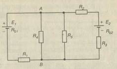 Fig.16 Fig.16 |
|
| Option No. | Data for calculations | Electrical circuit diagram |
| E 1 \u003d 90V; E 2 \u003d 120V; R 1 \u003d 4 Ohm; R 2 \u003d 29 Ohm; R 3 \u003d 30 Ohm; R 4 \u003d 10 Ohm; r 1 \u003d 1 Ohm; r 2 \u003d 1 Ohm. | 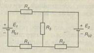 Fig.17 Fig.17 |
|
| E 1 \u003d 120V; E 2 \u003d 144V; R 1 \u003d 3.6 Ohm; R 2 \u003d 6.4 Ohm; R 3 \u003d 6 ohms; R 4 \u003d 4 Ohm r 1 \u003d 0.4 Ohm; r 2 \u003d 1.6 Ohm. |  Fig.18 Fig.18 |
|
| E 1 \u003d 160V; E 2 \u003d 200V; R 1 \u003d 9 Ohm; R 2 \u003d 19 Ohm; R 3 \u003d 25 Ohm; R 4 \u003d 100 Ohm; r 1 \u003d 1 Ohm; r 2 \u003d 1 Ohm. |  Fig.19 Fig.19 |
|
| E 1 \u003d 60V; E 2 \u003d 72V; R 1 \u003d 1.8 Ohm; R 2 \u003d 3.2 Ohm; R 3 \u003d 3 Ohm; R 4 \u003d 2 Ohm; r 1 \u003d 0.2 Ohm; r 2 \u003d 0.8 Ohm. | 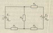 Fig.20 Fig.20 |
|
| E 1 \u003d 80V; E 2 \u003d 100V; R 1 \u003d 9 Ohm; R 2 \u003d 19 Ohm; R 3 \u003d 25 Ohm; R 4 \u003d 100 Ohm; r 1 \u003d 1 Ohm; r 2 \u003d 1 Ohm. | Rice. 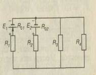 21 21
|
The solution of problem 2 requires knowledge of methods for calculating a complex electrical circuit and its sections, Kirchhoff's laws, methods for determining the equivalent circuit resistance. Before solving the problem, study the calculation methods for complex DC electrical circuits and consider typical examples corresponding to them.
Guidelines to solve problem 2:
2.1. Superimposed current method
The overlay method is one of the methods for calculating complex circuits with multiple sources.
The essence of the calculation of circuits by the overlay method is as follows:
1. In each branch of the circuit under consideration, the direction of the current is chosen arbitrarily.
2. The number of design circuits of the circuit is equal to the number of sources in the original circuit.
3. In each calculation scheme, only one source operates, and the remaining sources are replaced by their internal resistance.
4. In each design scheme, partial currents in each branch are determined by the folding method. Partial is a conditional current flowing in a branch under the action of only one source. The direction of partial currents in the branches is quite definite and depends on the polarity of the source.
5. The desired currents of each branch of the circuit under consideration are defined as the algebraic sum of partial currents for this branch. In this case, a partial current that coincides in direction with the desired one is considered positive, and a non-coinciding one is negative. If the algebraic sum has a positive sign, then the direction of the desired current in the branch coincides with the arbitrarily chosen one, if it is negative, then the direction of the current is opposite to the chosen one.
Example 2.1. Superimposed current method
Determine the currents in all branches of the circuit, the diagram of which is shown in Figure 22, if E 1 = 40 V is specified; E 2 \u003d 30 V; R 01 \u003d R 02 \u003d 0.4 Ohm; R 1 \u003d 30 Ohm; R 2 \u003d R 3 \u003d 10 Ohms; R 4 \u003d R 5 \u003d 3.6 ohms.
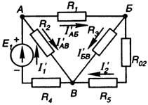
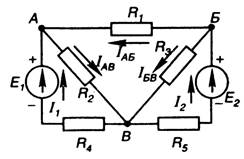
Figure 22 Figure 23
Figure 24
It is established that the number of branches and, accordingly, different currents in the circuit (Figure 22) is five, and the direction of these currents is arbitrarily chosen.
There are two calculation schemes, since there are two sources in the circuit.
The partial currents created in the branches by the first source (I’) are calculated. For this, the same circuit is depicted, only instead of E 2 - its internal resistance (R 02). The direction of partial currents in the branches is indicated in the diagram (Figure 23).
These currents are calculated by the convolution method
Then the first partial currents in the circuit (Figure 23) have the following values:
![]()
![]()
![]()
![]()
![]()
The partial currents generated by the second source (I'') are calculated. To do this, the original circuit is depicted, replacing the first source (E 1) in it with its internal resistance (R 01). The directions of these partial currents in the branches are shown in the diagram (Figure 24).
Let us calculate these currents using the convolution method.
The second partial currents in the circuit (Figure 24) have the following meanings:
![]()
![]()
![]()
![]()
![]()
Therefore, the desired currents in the circuit under consideration (Figure 22) are determined by the algebraic sum of partial currents (see Figures 22, 23 and 24) and have the following values:
The current I AB has a “-” sign, therefore, its direction is opposite to the arbitrarily chosen one, i.e. I AB is directed from point A to point B.
2.2. Nodal voltage method
The calculation of complex branched electrical circuits with several sources can be carried out using the nodal voltage method if there are only two nodes in this circuit. The voltage between these nodes is called nodal. U AB - nodal voltage of the circuit (Figure 25).
The value of the nodal voltage is determined by the ratio of the algebraic sum of the products of the EMF and the conductivity of the branches with sources to the sum of the conductivities of all branches:
To determine the signs of the algebraic sum, the direction of the currents in all branches is chosen the same, that is, from one node to another (Figure 25). Then the EMF of the source operating in the generator mode is taken with the “+” sign, and the source operating in the consumer mode is taken with the “-” sign.
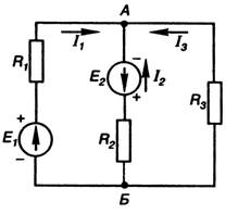 Figure 25
For the circuit shown in Figure 25, the nodal voltage is given by:
![]() ,
,
Where is the conductivity of the first branch; - conductivity of the second branch; is the conductivity of the third branch.
Nodal voltage (U AB) can be either positive or negative. Having determined the nodal voltage (U AB), you can calculate the currents in each branch.
Nodal voltage for the first leg:
Since the source E 1 operates in generator mode. Where
For the second branch, whose source E 2 operates in consumer mode:
For the third branch, since the conditionally chosen direction of the current I 3 indicates that point B () is greater than the potential of point A (). Then:
![]() ,
,
The “-” sign in the calculated current value indicates that the conditionally chosen current direction of this branch is opposite to the chosen one.
Example 2.2. Nodal voltage method
Figure 26
In the branches of the circuit (Figure 26), it is required to determine the currents if R 1 = 1.7 Ohm; R 01 \u003d 0.3 Ohm; R 2 \u003d 0.9 Ohm; R 02 \u003d 0.1 Ohm; R 3 \u003d 4 ohms; E 1 = 35 V; E 2 \u003d 70 V.
Determine the nodal voltage U AB
![]()
Where ; ; ![]() ;
;
![]()
We determine the currents in the branches:
As can be seen, the direction of the currents I 1 and I 3 is opposite to the chosen one. Therefore, the source E 1 operates in consumer mode.
2.3. Method of nodal and contour equations
Kirchhoff's laws underlie the calculation of complex electrical circuits by the method of nodal and contour equations.
The compilation of a system of equations according to Kirchhoff's laws (by the method of nodal and contour equations) is carried out in the following order:
1. The number of equations is equal to the number of currents in the circuit (the number of currents is equal to the number of branches in the calculated circuit). The direction of the currents in the branches is chosen arbitrarily.
2. According to the first Kirchhoff law, (n-1) equations are compiled, where n is the number of nodal points in the scheme.
3. The remaining equations are compiled according to the second Kirchhoff law.
As a result of solving the system of equations, we determine the desired values for a complex electrical circuit (for example, all currents for given values of the EMF of sources E and resistances of resistors R). If, as a result of the calculation, any currents turn out to be negative, this indicates that their direction is opposite to the chosen one.
Example 2.3. Method of nodal and contour equations

Figure 27
Compile the necessary and sufficient number of equations according to Kirchhoff's laws to determine all currents in the circuit (Figure 27) using the method of nodal and contour equations.
Solution. In the complex circuit under consideration, there are 5 branches, and, consequently, 5 different currents, therefore, for the calculation it is necessary to compose 5 equations, and two equations according to the first Kirchhoff law (in the circuit n \u003d 3 nodal points A, B and C) and three equations - according to Kirchhoff's second law (we go around the circuit clockwise and neglect the internal resistance of the sources, i.e. R 0 \u003d 0). We make equations:
1) (for point A)
2) ![]() (for point B)
(for point B)
3) (for circuit A, a, B)
4) (for circuit A, B, b, C)
5) (for circuit A, B, c)
We go around the contours clockwise.
2.4. Loop current method
 When calculating complex circuits by the method of nodal and contour equations (according to Kirchhoff's laws), it is necessary to solve a system of a large number of equations, which greatly complicates the calculations. So for the circuit (Figure 28) it is necessary to compile and calculate a system composed of 7 equations (according to Kirchhoff's laws).
Figure 28
For this purpose, we select m independent circuits in the circuit, in each of which we arbitrarily direct the circuit current (I I, I II, I III, I IV). The loop current is a calculated value that cannot be measured. As you can see, the individual branches of the circuit are included in two adjacent circuits. Then the real current in such a branch is determined by the algebraic sum of the loop currents of adjacent loops:
To determine the loop currents, we compose m equations according to the second Kirchhoff law. Each equation includes the algebraic sum of the emfs included in this circuit (on one side of the equals sign) and the total voltage drop in this circuit created by the circuit current of this circuit and the circuit currents of adjacent circuits (on the other side of the equals sign).
Thus, for the circuit (Figure 28), we compose 4 equations. With a plus sign, EMF and voltage drops (on opposite sides of the equal sign) are recorded, acting in the direction of the loop current, with a minus sign, directed against the loop current
Having determined the loop currents, having calculated the system of equations, we calculate the real currents in the circuit under consideration.
Example 2.4. Loop current method
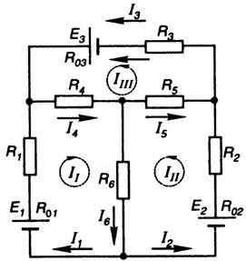
Figure 29
Determine the currents in all sections of the complex circuit (Figure 29), if E 1 \u003d 130 V; E 2 \u003d 40 V; E 3 \u003d 100 V; R 1 \u003d 1 Ohm; R 2 \u003d 4.5 ohms; R 3 \u003d\u003d 2 Ohm; R 4 \u003d 4 ohms; R 5 \u003d 10 Ohm; R 6 \u003d 5 ohms; R 02 \u003d 0.5 0m "R 01 \u003d R 03 \u003d O Ohm.
2. Errors. Classification of errors; their causes, methods of detection and solutions.
Option 3
1. Metals and alloys, application in solders. Solder marking. Conditions and factors influencing the choice of solder brand.
2. Device, typical parts and assemblies of indicating electrical measuring instruments.
Option 4
1. Electrical strength of dielectrics. Methods and devices for testing electrical strength.
2. The principle of operation, device and scope of measuring mechanisms and devices of the magnetoelectric system.
Option 5
1. Thermal characteristics ETM: melting point, flash point and softening of materials, heat resistance, frost resistance, resistance to thermal shocks, temperature coefficients.
2. The principle of operation, device and scope of measuring mechanisms and devices of the electromagnetic system.
Option 6
1. Physical and chemical characteristics: acid number, viscosity, moisture resistance, chemical resistance, tropical resistance, radiation resistance of materials.
2. Principles of operation, device, switching circuits and scope of measuring mechanisms and devices of electrodynamic systems.
Option 7
1. Conducting copper. Receiving copper. Physical, mechanical and electrical properties of copper. Soft copper. Solid copper. Copper grades according to GOST. The use of copper.
2. Principles of operation, device, switching circuits and scope of measuring mechanisms and devices of the ferrodynamic system.
Option 8
1. Contact definition. Fixed, breaking and sliding contacts, their device. Requirements for contact materials.
2. Principles of operation, device, switching circuits and scope of measuring mechanisms and devices of the induction system.
Option 9
1. High resistance alloys: manganin, constantan, nichrome, fechral. Their properties, grades according to GOST and application.
2. Magnetoelectric measuring mechanisms with transducers: thermoelectric devices, rectifying devices, vibrational and ratiometric.
Option 10
1. Refractory materials tungsten and molybdenum, their properties and applications.
2. Dynamic characteristics of ETM: vibration strength and impact strength. Standard samples, devices and test methods.
CONTROL WORK №2
Electric magnetic phenomena were known in ancient times, but the beginning of the development of the science of these phenomena (electrical engineering) is considered to be 1600. This year, the English physicist W. Hilbert published the results of some studies of electrical and magnetic phenomena, introduced the term "electricity". The theory of atmospheric electricity (the field of static electricity) was published in 1753 by M.V. Lomonosov. In 1785, S. Coulomb established the law of interaction of electric charges, in 1800, A. Volta invented a galvanic cell. Further, the number of discoveries of new laws, theories, inventions began to increase rapidly. Such scientists as V.V. Petrov, H. Oersted, A. Ampere, M. Faraday, E.Kh. Lenz, B.S. Jacobi, D. Maxwell, A.G. Stoletov, V.N. Chikalev, P.N. Yablochkov, M.O. Dolivo-Dobrovolsky and many others. Currently, entire institutes and research and production associations work in the field of electrical engineering. An international electrotechnical commission has been created, whose task is to determine standards for the receipt and use of electrical energy in various industries. Radio engineering and electronics and other branches of science got their start in the science of electrical engineering.
Definitions of the concept "Science of electrical engineering":
Electrical engineering is a science that deals with the use of the properties of an electromagnetic field to receive, transmit and convert electrical energy.
Electrical engineering as a science studies the properties of receiving, transmitting and converting electrical energy.
Electrical engineering is the science of processes associated with the practical application of electrical and magnetic phenomena.
Electrical engineering as a science is a field of knowledge that deals with electrical and magnetic phenomena and their practical use.
Electrical engineering as a science is a basic discipline for studying special disciplines such as radio engineering, radio circuits and signals, secondary power supplies, and others.
Energy is a quantitative measure of the movement and interaction of all forms of matter .
For any kind of energy, one can name a material object that is its carrier. The carrier of electrical energy is the electromagnetic field.
Electrical energy has found wide application due to its properties:
universality, i.e. easily converted into other non-electric types of energy and vice versa;
transmitted over long distances with little loss;
easily crushed and distributed among consumers of various capacities
Easily adjustable and controlled by various devices.
Electrical energy is used in all industries without exception and Agriculture, in science, in medicine, in the service industries and, of course, in everyday life.
Radio engineering as a science solves the problems of using an electromagnetic field and electrical energy to transmit information without wires.
BASIC LAWS OF ELECTRICAL ENGINEERING
Topic1.1
Basic information about the electric field, conductors, semiconductors,
Common in electrical circuits mixed connection, which is a combination of serial and parallel connections. If we take, for example, three devices, then two options for a mixed connection are possible. In one case, two devices are connected in parallel, and a third is connected in series to them (Fig. 1, a).
Such a circuit has two sections connected in series, one of which is parallel connection. According to another scheme, two devices are connected in series, and a third one is connected to them in parallel (Fig. 1, b). This circuit should be considered as a parallel connection in which one branch is itself a series connection.
With more devices, there may be different, more complex mixed connection schemes. Sometimes there are more complex circuits containing several sources of emf.
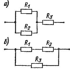
Rice. 1. Mixed connection of resistors
To calculate complex circuits, there are various methods. The most common of these is the application. In the very general view this law states that in any closed loop, the algebraic sum of the EMF is equal to the algebraic sum of the voltage drops.
It is necessary to take the algebraic sum because the EMF acting towards each other, or the voltage drops created by oppositely directed currents, have different signs.
When calculating a complex circuit, in most cases, the resistances of individual sections of the circuit and the EMF of the included sources are known. To find the currents, one should, in accordance with the second Kirchhoff's law, formulate equations for closed circuits in which the currents are unknown quantities. To these equations, we must add the equations for branching points, compiled according to the first Kirchhoff law. Solving this system of equations, we determine the currents. Of course, for more complex circuits, this method turns out to be rather cumbersome, since it is necessary to solve a system of equations with a large number of unknowns.
The application of Kirchhoff's second law can be shown by the following simple examples.
Example 1. An electrical circuit is given (Fig. 2). The EMF of the sources are E1= 10 V and E2 = 4 V, and r1 = 2 Ω and r2 = 1 Ω, respectively. EMF sources act towards. Load resistance R = 12 Ohm. Find current I in the chain.

Rice. 2. Electric circuit with two sources connected towards each other
Solution. Since in this case there is only one closed loop, we make up one single equation: E 1 - E 2 \u003d IR + Ir 1 + Ir 2.
On the left side we have the algebraic sum of the EMF, and on the right side - the sum of the voltage drops created by the current I on all sequentially included sections R, r1 and r2.
Otherwise, the equation can be written like this:
E1 - E2 = I (R = r1 + r2)
Or I = (E1 - E2) / (R + r1 + r2)
Substituting numerical values, we get: I \u003d (10 - 4) / (12 + 2 + 1) \u003d 6/15 \u003d 0.4 A.
This problem, of course, could be solved on the basis of , bearing in mind that when two EMF sources are turned on towards each other, the effective EMF is equal to the difference E 1 - E2, in the total resistance of the circuit is the sum of the resistances of all the included devices.
Example 2. A more complex scheme is shown in fig. 3.

Rice. 3. Parallel operation of sources with different emfs
At first glance, it seems quite simple. Two sources (for example, a DC generator and a battery are taken) are connected in parallel and a light bulb is connected to them. The EMF and internal resistances of the sources are respectively equal: E1 = 12 V, E2 = 9 V, r1 = 0.3 ohm, r2 = 1 ohm. Bulb resistance R \u003d 3 Ohm It is necessary to find currents I1, I2 , I and voltage U at the source terminals.
Since the EMF E 1 greater than E2, then in this case the generator E1 obviously charges the battery and powers the bulb at the same time. We compose equations according to the second Kirchhoff law.
For a circuit consisting of both sources, E1 - E2 = I1rl = I2r2.
The equation for a circuit consisting of a generator E1 and a light bulb is E1 = I1rl + I2r2.
And, finally, in the circuit, which includes the battery and the light bulb, the currents are directed towards each other and therefore for it E2 = IR - I2r2. These three equations are not sufficient to determine the currents, since only two of them are independent, and the third can be obtained from the other two. Therefore, you need to take any two of these equations and write the equation according to the first Kirchhoff law as the third one: I1 = I2 + I.
Substituting the numerical values of the quantities into the equations and solving them together, we get: I1 \u003d 5 A, I 2 \u003d 1.5 A, I \u003d 3.5 A, U \u003d 10.5 V.
The voltage at the generator terminals is 1.5 V less than its EMF, since a current of 5 A creates a voltage loss of 1.5 V per internal resistance r1 = 0.3 ohm. But the voltage at the terminals battery more than its EMF by 1.5 V, because the battery is charged with a current equal to 1.5 A. This current creates a voltage drop of 1.5 V on the internal resistance of the battery (r2 \u003d 1 Ohm), and it is added to the EMF.
Don't think that stress U will always be the arithmetic mean of E 1 and E2, as it turned out in this particular case. It can only be argued that in any case U must be between E1 and E2.
Analysis of complex DC electrical circuits.
Method of Kirchhoff's Laws
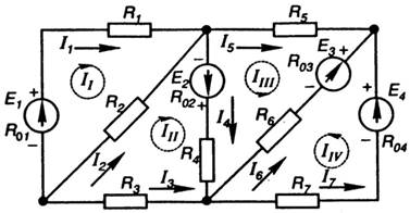
A complex electrical circuit is usually called a branched circuit containing several sources located in different branches. An example of a complex DC circuit is shown in fig. 22.
Rice. 22. An example of a complex DC circuit
The true directions of currents in the branches of a complex electrical circuit, as a rule, are unknown. Therefore, the analysis of a complex circuit begins with the choice of the so-called positive directions of currents in the branches of the circuit. In the diagram, the positive directions of currents in the branches are indicated by arrows with current symbols I. An example of the choice of conditional positive directions of currents in the branches of the circuit is shown in fig. 22.
If, as a result of circuit analysis, it turns out that the current in the branch is positive, then the true direction of the current will coincide with the selected positive direction of the current. If, as a result of the calculation, it turns out that the current in the branch is negative, then the true direction of the current is opposite to the chosen positive direction of the current. Those. during the analysis of the electrical circuit, the currents in the branches are considered as algebraic quantities.
The most general approach to the analysis of complex electrical circuits is based on the use of Kirchhoff's laws. With the help of Kirchhoff's laws, a system of linear algebraic equations relative to unknown currents. The number of unknown currents is equal to the number of circuit branches. Let's denote this number by m. Therefore, with the help of Kirchhoff's laws, it is necessary to compose a system of m equations with m unknown currents.
When compiling equations according to Kirchhoff's laws, it is necessary to adhere to next rule. If in the diagram n knots, then with the help of the first Kirchhoff law, ( n– 1) independent equation. (The equation for the last node will be dependent). Remaining [ m–(n–1)] equations are compiled using the second Kirchhoff law for the so-called independent circuits.
Independent Circuit- this is such a contour, when traversing which, at least one new branch appears in comparison with the previously considered contours.
In a branched circuit, the number of independent circuits is always less than the total number of circuits. Therefore, when choosing independent circuits, there is a certain freedom of choice. However, the number of independent circuits in the circuit is always regulated. Scheme fig. 22, for example, contains
[m– (n – 1)] = = 3
independent contours.
As a result of compiling ( n– 1) equations according to the first Kirchhoff law and [ m– (n– 1)] of the equation according to the second Kirchhoff law, a system is formed from m equations for unknown branch currents. The solution of this system makes it possible to determine the branch currents.
Scheme fig. 22 consists of six branches. The selected positive directions of currents in the branches are indicated on the diagram by arrows with current symbols I 1 , I 2 , I 3 ,I 4 , I 5 , I 6 . To calculate the currents in the branches of this circuit using Kirchhoff's laws, it is necessary to compose a system of six equations.
The circuit contains four nodes ( n= 4). According to Kirchhoff's first law, three equations must be composed. Let us agree, when compiling equations according to the first Kirchhoff law, to take the currents leaving the node under consideration with the plus sign, and those entering the node with the minus sign.
In knot A enter current I 1 , and currents come out I 2 and I 3 . Then for the node a the equation of the first Kirchhoff law will have the form
![]()
From node b currents come out I 1 , I 4 , I 6 . Kirchhoff's first law equation for a knot b has the form
![]()
In knot c includes currents I 2 and I 4, and the current comes out I 5 . Therefore, for the node c can be written
![]()
Kirchhoff's First Law Equations Compiled for Knots A, b, c, include the currents of all six branches of the circuit under consideration. Summing up the equations compiled according to the first Kirchhoff law for knots A, b, c, we get the following equation:
![]()
This equation differs from the first Kirchhoff law equation for the knot d only signs, namely:
![]()
That is, the equation of the first Kirchhoff law for the node d dependent.
According to Kirchhoff's second law, for the circuit under consideration, it is necessary to compose three equations for three independent circuits. As independent circuits, for example, the left circuit composed of the first, second and fourth branches, the right circuit composed of the second, third and fifth branches, and the lower circuit composed of the fourth, fifth and sixth branches can be considered.
When compiling the equation of the second Kirchhoff law for each independent circuit, it is necessary to adhere to the following rule. If the chosen positive direction of the current in the branch coincides with the direction of the circuit bypass, then the voltage drop on the corresponding element R on the left side of the equation of the second Kirchhoff law is taken with a plus sign. If the chosen positive direction of the current in the branch is opposite to the direction of bypassing the circuit, then the voltage drop on the corresponding element R on the left side of the equation of the second Kirchhoff law is taken with a minus sign. If the direction of action of the EMF source, indicated by the arrow in the diagram, coincides with the direction of bypassing the circuit, then the corresponding EMF E on the right side of the equation of the second Kirchhoff law is taken with a plus sign. If the direction of the EMF source, indicated by the arrow in the diagram, is opposite to the direction of bypassing the circuit, then the corresponding EMF E on the right side of the equation of the second Kirchhoff law is taken with a minus sign.
Directions for bypassing independent circuits in the diagram of fig. 22 will be chosen clockwise. These bypass directions are indicated in the diagram by arrows that close along each of the independent contours.
Consider each of the independent circuits in turn. In the left circuit currents I 1 and I 2 coincide with the direction of bypassing the contour. Voltage drops R 1 I 1 , R 2 I 2 on the left side of the equation of the second Kirchhoff law for the left circuit must be taken with a plus sign. Current I 4 has a direction opposite to the direction of bypassing the left contour. Voltage drop R 4 I 4 on the left side of the equation of the second Kirchhoff law for the left contour must be taken with a minus sign. Direction of action of the EMF source E 1 is the same as the direction of the loop. On the right side of the equation of the second Kirchhoff law, the EMF E 1 must be taken with a plus sign. Directions of action of EMF sources E 2 and E 4 are opposite to the direction of bypassing the contour. On the right side of the equation of the second Kirchhoff law, the EMF E 2 and E 4 must be taken with a minus sign. Thus, for the left independent contour, the following equation of the second Kirchhoff law is valid:
Similarly, for the right and lower independent circuits of the circuit in Fig. 22 we obtain the following equations of the second Kirchhoff law:
When combining the equations compiled according to the first and second Kirchhoff laws for the scheme of Fig. 22, the following system of linear algebraic equations is obtained:
The solution of this system allows us to find the currents I 1 , I 2 , I 3 ,I 4 , I 5 , I 6 . Known currents can be used to find voltage drops on circuit elements, power, and so on.
The stated method of analyzing complex electrical circuits is called the method of Kirchhoff's laws. The method of Kirchhoff's laws is the most general approach to the analysis of electrical circuits.
Other methods can be used to analyze complex electrical circuits, for example, the loop current method, the nodal potential method, the superposition method, the equivalent generator method. These methods are based on Kirchhoff's laws, Ohm's law, and the superposition principle. Therefore, they are valid for linear circuits. An exception is the equivalent generator method, which assumes that the branch with the desired current can also be non-linear. The variety of methods for analyzing complex electrical circuits allows in each specific case choose the method that gives the simplest calculation algorithm.
In particular, the method of loop currents and the method of nodal potentials, like the method of Kirchhoff's laws, are reduced to solving systems of linear algebraic equations. However, the number of required quantities, and, consequently, the order of systems of linear algebraic equations in these methods is less than in the method of Kirchhoff's laws.
Known mathematical methods are used to solve systems of linear algebraic equations. With a small number of equations in the system, the method of determinants (Cramer's rule) can be used. When enough in large numbers equations in the system, it is advisable to use the method of successive elimination unknown gauss with the choice of the main element or iterative methods for solving systems of linear algebraic equations, for example, the Seidel method.
The correctness of the obtained solution can be verified by substituting the found values of the branch currents into a system of equations compiled according to Kirchhoff's laws, or by compiling a power balance (see below).
Consider in turn the main methods of analysis of electrical circuits. But first consider general question relating to the geometric structure of electrical circuits.
 (1 ratings, on average: 5,00 out of 5)