Construct high-quality graphs of the currents indicated on the diagram. What are vector diagrams and what are they for?
Application of vector diagrams in the calculation and study of electronic circuits alternating current allows you to clearly present the processes under consideration and simplify the electrical calculations performed.
Vector diagrams are a set of vectors depicting the operating sinusoidal emf and currents or their amplitude values.
A harmonically varying voltage is given by u = U m sin ( ωt + ψ and).
Place it at an angle ψ and relative to the positive x-axis x vector U m, the length of which on an arbitrarily chosen scale is equal to the amplitude of the depicted harmonic quantity (Fig. 1). We will plot positive angles in a counterclockwise direction, and negative angles in a clockwise direction. Let's imagine that the vector U m, starting from time t = 0, rotates around the origin of coordinates counterclockwise with a constant rotation frequency ω equal to the angular frequency of the depicted voltage. At time t, vector Um will rotate through an angle ωt and will be placed at an angle ωt + ψ and in relation to the abscissa axis. The projection of this vector onto the ordinate axis on a selected scale is equal to the instantaneous value of the depicted voltage: u = U m sin ( ωt + ψ and).

Rice. 1. Rotating vector sinusoidal voltage image
As follows, a quantity that varies harmoniously with time can be represented rotating vector. With the initial phase equal to zero, when u = 0, the vector U m for t = 0 must be placed on the x-axis.
A graph of the dependence of any variable (including harmonic) quantity on time is called time diagram. For harmonic quantities, it is more convenient to plot along the abscissa axis not the time t itself, but the value proportional to it ω t. Timing diagrams absolutely define the harmonic function because they give an idea of the initial phase, amplitude and period.
Usually, when calculating a circuit, we are only interested in the effective EMF, voltages and currents, or the amplitudes of these quantities, as well as their phase shift relative to each other. Therefore, fixed vectors are usually considered for a certain moment in time, which is chosen so that the diagram is pleasant. This diagram is called vector diagram. With all this phase shift angles are plotted in the direction of rotation of the vectors (counterclockwise) if they are positive, and in the opposite direction if they are negative.
If, for example, the initial phase angle of the voltage ψ and greater than the initial phase angle ψi then the phase shift φ = ψ and— ψ i and this angle is plotted in the positive direction from the current vector.
When calculating an alternating current circuit, it is often necessary to calculate the emf, currents or voltages of the same frequency.
Let's imagine that we need to add two emfs: e 1 = E 1 m sin ( ωt + ψ 1e ) and e 2 = E 2m sin ( ωt + ψ 2e).
This addition can be done analytically and graphically. The last method is more visual and simple. Two folded emfs e 1 and e 2 on a certain scale are represented by the vectors E 1 m E 2m (Fig. 2). When these vectors rotate with the same rotation frequency, equal to the angular frequency, the mutual placement of the rotating vectors remains constant.
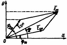
Rice. 2. Graphic addition of 2 sinusoidal EMFs of similar frequency
The sum of the projections of the rotating vectors E 1 m and E 2m onto the ordinate axis is equal to the projection onto the same axis of the vector E m, which is their geometric sum. As follows, when two sinusoidal EMFs of the same frequency are added, a sinusoidal EMF of the same frequency comes out, the amplitude of which is represented by the vector Em equal to the geometric sum of the vectors E 1 m and E 2m: E m = E 1 m + E 2m.
Vectors of alternating emfs and currents are graphical representations of emfs and currents, in contrast to vectors physical quantities, having a certain physical meaning: force vector, field strength and others.
The indicated method can be used to add and subtract any number of emfs and currents of the same frequency. The subtraction of 2 sinusoidal quantities can be represented in the form of addition: e 1 - e 2 = e 1 + (- e 2), i.e., the quantity being reduced is added to the subtrahend, taken with the opposite sign. Typically, vector diagrams are not built for amplitude values alternating emfs and currents, but for effective quantities proportional to amplitude values, because all circuit calculations are usually made for effective emfs and currents.
Electrician school
When circuit elements are connected in series, the same current I flows through each of them. Therefore, when constructing vector diagrams for such circuits, the current vector is taken as the base (initial) one. Vector diagrams are constructed using a compass using the notching method using voltages known from experience: U a - at the resistor terminals, U k - at the coil terminals, U c - at the capacitor terminals and U - at the terminals of the entire circuit. All values in the diagrams are shown to scale.
As an example, consider constructing a vector diagram for a circuit with serial connection resistor (rheostat) and coil. The voltage across the resistor U a , which is in phase with the current I, is scaled along the current line. From the end of the vector with radius, equal to voltage on the coil U k, make the first notch. The second notch is made with a radius equal to the total circuit voltage U from the beginning of the vector. At the intersection point of the serifs there will be the ends of the vectors and (Fig. 3.14.a). The active and inductive components of the voltages on the coil are determined by dropping a perpendicular to the axis of the current vector İ from the end of the vector.
The vector diagram for a circuit with a series connection of a coil and a capacitor is constructed in a similar way and is shown in Fig. 3.14.b.
 |
 a b
a b
Rice. 3.14. Constructing vector diagrams using the serif method.
 |
Rice. 3.15. Connection diagram of electrical circuit with serial
turning on the coil and capacitor bank.
The order of work.
1. Assemble the electrical circuit according to the diagram in Fig. 3.15.
2. Carry out a study of the phenomenon of voltage resonance using the following method.
By changing the value of the capacitance by turning on the toggle switches, set the capacitance C 0 at which the current in the circuit I and active power P have maximum values (a phenomenon close to voltage resonance). Measure the voltage U in the circuit, the voltage on the coil U k, the voltage on the capacitor U c, the current I in the circuit and the power P. Then changing the capacitance in steps of 1 - 2 μF, take measurements for 3 - 4 points with capacitances less than C 0 , and for 3 – 4 points with capacities larger than C 0.
3. Enter the measurement results for each installed capacity value in Table 3.1.
Table 3.1
4. Based on the experimental data, calculate the values indicated in table. 3.1 (circuit impedance Z, active resistance r, reactance x, circuit power factor cosφ, capacitance x C, capacitance C, coil impedance z k, coil inductive reactance z L, coil inductance L, power factor cosφ k).
Formulas for calculations
; ; ; ;
; ; ; ![]()
;
5. According to table. 3.1 construct the curves I=f 1 (C), cosφ=f 2 (C); z=f 3 (C).
6. Construct vector diagrams of current and voltage for three readings: at x L >x C, at the maximum current value in the circuit (x L ≈x C), at x L Control questions:
1. What is called inductive and capacitive reactance and what do they depend on? 2. How is the impedance of an unbranched AC circuit calculated? 3. How is the effective current value calculated in a circuit with a series connection of resistive, inductive and capacitive elements? 4. What is the power factor of an AC circuit and why should we strive to increase it when consuming electrical energy? 5. Under what condition does voltage resonance occur in an alternating sinusoidal current circuit? How is this phenomenon characterized? 6. Explain what danger voltage resonance in electrical circuits can pose? 7. What should be the ratio of inductive and capacitive reactance so that the current in the circuit is ahead of the voltage? Explain this with the help of a vector diagram. 8. What additionally needs to be included in this circuit in order to obtain voltage resonance in it? 9. In an alternating current circuit with a frequency of f=50 Hz with a coil and capacitor connected in series, resonance occurs. Determine the voltage on the coil and capacitor if U=20V, r=10Ohm, c=1uF. Calculate the inductance of the coil. Work 4. Parallel connection of inductance and capacitance. Resonance of currents. Goal of the work: consider the phenomena occurring in an alternating current circuit containing a coil and a capacitor connected in parallel (Fig. 4.1), become familiar with the resonance of currents. Rice. 4.1. Circuit diagram with parallel connection of elements. Explanations for work Let's consider a parallel connection of a coil with inductive x L =ωL and active r resistances with a capacitor with capacitive reactance (Fig. 4.2). When such a circuit is turned on under voltage U, a current Ic appears in the coil. Rice. 4.2. Schematic diagram of parallel connections r, x L, x c Where The current vector will lag behind the voltage vector by an angle φ to: ; A current I c arises in the capacitor: The current vector İ c will be 90˚ ahead of the vector, φ c = 90˚. The total current vector based on Kirchhoff's first law: İ = İ k + İ s. (4.4) The vector diagram of currents according to (4.4) is shown in Fig. 4.3 The current vector İ k is drawn at an angle φ k to the voltage vector. From the end of the current vector İ to we draw the current vector İ c at an angle φ c = 90˚ to the voltage vector (in the leading direction). The sum of the vector İ k and İ c will give the total current vector, which lags behind the voltage vector by an angle φ. To analytically determine the total current I and the angle φ, we decompose the coil current I k into the active component I a, coinciding with the voltage U, and the inductance I L, lagging 90˚ from the voltage U. Dividing the sides of the triangle (Fig. 4.3) by the voltage U, we obtain a conductivity triangle (Fig. 4.4), from which we find: By changing the value of capacitance C, on which the value of b c depends, according to (4.7), you can change the relationship between b c and inductive conductances (b L), and, consequently, currents: I c =Ub c =Uωс; I L =Ub L Fig.4.3. Vector diagram of voltage and current for a circuit with parallel connecting the coil and capacitance at I L >I C At b C
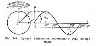
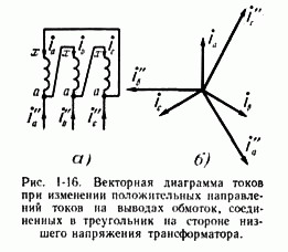
Uωс Inductive conductivity b L and, consequently, current I L predominate, therefore the total current vector İ lags behind the voltage vector (Fig. 4.3). When b C > b L , i.e. C> we have: Uωс Capacitive conductivity b C and, consequently, current I C predominate, therefore the total current vector İ is ahead of the voltage vector (Fig. 4.5). Fig.4.4. connection of the coil and capacitance at I C< I L Fig.4.5. Vector diagram for a circuit with parallel connecting the coil and capacitance at I C > I L With a capacitance value: , (4.12) capacitive conductivity is equal to inductive conductivity: b C = ωc = b L , (4.13) and, therefore, the capacitive and inductive currents will be equal to each other (Fig. 4.6): b C U= b L U ; I C = I L . (4.14) We will get a current resonance, i.e. complete mutual compensation of inductive and capacitive currents: I C – I L = 0. (4.15) As a result, the total current I at resonance consists only of the active component, according to expression (4.8) and Fig. 4.6. I= I a = Ug, (4.16) therefore angle φ= 0, and cos φ= 1. The total conductance of the circuit, and therefore the current I, takes a minimum value, since according to (4.10) У = g, since b C – b L = 0, and the total resistance of the circuit is, therefore, the maximum value. The reactive power of the circuit is zero: U(I C - I L) = 0 ; Q L – Q C = 0. Fig.4.6. Vector diagram for current resonance (IC = I L) The phenomenon of current resonance, i.e. mutual compensation of reactive currents (I C –I L =0), and, consequently, reactive powers (Q L –Q C =0) is explained as follows. When the inductive branch (coil) consumes energy to create a magnetic field, at that moment the capacitor in the parallel branch discharges and releases energy. Mutual compensation of energies occurs. The total energy consumed from the network is spent only on the active resistance of the coil (for heating the coil wire). The dependence of the total resistance Z of the circuit on the capacitance value will have the following form: where and do not depend on C. Fig.4.7. Graph of current in circuit I, cosφ and total resistance z from the capacitance. a) The concept of vectors In Fig. 1-4 shows a curve of changes in alternating current over time. The current first increases from zero (at = 0°) to the maximum positive value + I M (at = 90°), then decreases, passes through zero (at = 180°), reaches the maximum negative value - I M (at = 270°) and finally returns to zero (at = 360°). After this, the entire cycle of current change is repeated. The curve of changes in alternating current over time, plotted in Fig. 1-4 is called a sine wave. The time T during which a complete cycle of current change occurs, corresponding to an angle change of up to 360°, is called the period of alternating current. The number of periods in 1 s is called the frequency of alternating current. In industrial installations and in everyday life in the USSR and other European countries, alternating current with a frequency of 50 Hz is mainly used. This current takes on a positive and negative direction 50 times per second. The change in alternating current over time can be written as follows: where i is the instantaneous value of the current, i.e. the value of the current at each moment of time; I m - maximum current value; - angular frequency of alternating current, f= 50 Hz, = 314; - the initial angle corresponding to the moment in time from which the time count begins (at t = 0). For the special case shown in Fig. 1-4, When analyzing the operation of relay protection and automation devices, it is necessary to compare currents and voltages, add or subtract them, determine the angles between them and perform other operations. Use curves similar to those shown in Fig. 1-4 is inconvenient, since constructing current and voltage sinusoids takes a lot of time and does not give a simple and clear result. Therefore, for simplicity, it is customary to depict currents and voltages in the form of straight line segments having a certain length and direction - the so-called vectors (OA in Fig. 1-4). One end of the vector is fixed at point O - the origin of coordinates, and the second rotates counterclockwise. The instantaneous value of current or voltage at each moment of time is determined by the projection onto vertical axis a vector whose length is equal to the maximum value of the electrical value of current or voltage. This projection will become either positive or negative, taking maximum values when the vector is vertical. During a time T equal to the period of the alternating current, the vector will make a complete revolution around the circle (360°), occupying sequential positions, etc. At an alternating current frequency of 50 Hz, the vector will make 50 rps. Thus, the current or voltage vector is a straight line segment, equal in magnitude to the maximum value of the current or voltage, rotating relative to point O counterclockwise at a speed determined by the frequency of the alternating current. Knowing the position of the vector at each moment of time, it is possible to determine the instantaneous value of the current or voltage at a given moment. So, for the position of the current vector OA shown in Fig. 1-5, its instantaneous value is determined by the projection onto the vertical axis, i.e. Based on Fig. 1-5, we can also say that the current at a given time has a positive value. However, this does not yet give a complete picture of the process in an alternating current circuit, since it is not known what positive or negative current, positive or negative voltage means. In order for vector diagrams of currents and voltages to give a complete picture, they must be linked to the actual course of the process in the alternating current circuit, that is, it is necessary to first accept the conditional positive directions of currents and voltages in the circuit under consideration. Without this condition, if the positive directions of currents and voltages are not specified, any vector diagram has no meaning. Consider a simple single-phase AC circuit shown in Fig. 1-6, a. From a single-phase generator, energy is transferred to the active load resistance R. Let us set the positive directions of currents and voltages in the circuit under consideration. For the conditional positive direction of voltage and emf. we will take the direction when the potential of the generator or load output connected to the line is higher than the potential of the output connected to the ground. In accordance with the rules accepted in electrical engineering, the positive direction for e. d.s. indicated by an arrow pointing toward a higher potential (from ground to line terminal), and for voltage by an arrow pointing toward a lower potential (from line terminal to ground). Let's construct the vectors e. d.s. and current, characterizing the operation of the circuit under consideration (Fig. 1-6, b). Vector e. d.s. arbitrarily denoted by a vertical line with an arrow pointing upward. To construct the current vector, we write the equation for the circuit according to Kirchhoff’s second law: Since the signs of the current vectors and e. d.s. in expression (1-7) coincide, the current vector will coincide with the e vector. d.s. and in Fig. 1-6, b. Here and in the future, when constructing vectors, we will set them aside in magnitude equal to the effective value of current and voltage, which is convenient for performing various mathematical operations with vectors. As is known, the effective values of current and voltage are several times less than the corresponding maximum (amplitude) values. For given positive directions of current and voltage, the sign of the power is also uniquely determined. In the case under consideration, the power directed from the generator buses to the line will be considered positive: since the current vectors and e. d.s. in Fig. 1-6, b coincide. Similar considerations can be made for the three-phase alternating current circuit shown in Fig. 1-7, a. In this case, all phases have the same positive directions, which corresponds to the symmetrical diagram of currents and voltages shown in Fig. 1-7, b. Note that a three-phase system of vectors is called symmetrical when all three vectors are equal in magnitude and shifted relative to each other by an angle of 120°. Generally speaking, it is not at all necessary to take the same positive directions in all phases. However, it is inconvenient to accept different positive directions in different phases, since it would be necessary to depict an asymmetrical system of vectors when the electrical circuit operates in a normal symmetrical mode, when all three phases are under the same conditions. b) Operations with vectors When we consider only one current or voltage curve, the initial value of the angle from which the count begins, or, in other words, the position of the vector on the diagram corresponding to the initial moment of time, can be taken arbitrary. If two or more currents and voltages are simultaneously considered, then, having given the initial position on the diagram of one of the vectors, we thereby already determine the position of all other vectors. All three vectors phase voltages shown in Fig. 1-7, b, rotate counterclockwise at the same speed, determined by the frequency of the alternating current. At the same time, they intersect the vertical axis, which coincides with the direction of the vector in Fig. 1-7,b, alternately with a certain sequence, namely which is called the alternation of voltage (or current) phases. In order to determine mutual arrangement two vectors, one is usually said to be ahead or behind the other. In this case, the leading vector is the one that, when rotating counterclockwise, crosses the vertical axis earlier. So, for example, we can say that the voltage vector in Fig. 1-7, b leads by an angle of 120°, or, on the other hand, the vector lags behind the vector by an angle of 120°. As can be seen from Fig. 1-7, the expression “the vector lags behind by an angle of 120°” is equivalent to the expression “the vector leads by an angle of 240°”. When analyzing different electrical circuits, it becomes necessary to add or subtract current and voltage vectors. The addition of vectors is carried out by geometric summation according to the parallelogram rule, as shown in Fig. 1-8, a, on which the sum of currents is based Since subtraction is the inverse action of addition, it is obvious that to determine the current difference (for example, it is enough to add the inverse vector to the current At the same time, in Fig. 1-8, and it is shown that the current difference vector can be constructed more simply by connecting the ends of the vectors with a line. In this case, the arrow of the current difference vector is directed towards the first vector, i.e. A vector diagram of phase-to-phase voltages is constructed in exactly the same way, for example Obviously, the position of a vector on the plane is determined by its projections onto any two axes. So, for example, in order to determine the position of the vector OA (Fig. 1-9), it is enough to know its projections onto mutually perpendicular axes Let us plot the projections of the vector and on the coordinate axes and restore perpendiculars to the axes from the points. The intersection point of these perpendiculars is point A - one end of the vector, the second end of which is point O - the origin of coordinates. c) Purpose of vector diagrams Workers involved in the design and operation of relay protection very often have to use in their work so-called vector diagrams - current and voltage vectors plotted on a plane in a certain combination corresponding to the electrical processes occurring in the circuit under consideration. Vector diagrams of currents and voltages are constructed when calculating short circuits and when analyzing current distribution in normal mode. Analysis of vector diagrams of currents and voltages is one of the main, and in some cases, the only way to check the correct connection of current and voltage circuits and the activation of relays in differential and directional protection circuits. In fact, constructing a vector diagram is advisable in all cases when two or more electrical quantities are supplied to the relay in question: the current difference in overcurrent or differential protection, current and voltage in a power direction relay or in a directional resistance relay. The vector diagram allows you to draw a conclusion about how the protection in question will work in the event of a short circuit, i.e., evaluate the correctness of its activation. The relative position of the current and voltage vectors on the diagram is determined by the characteristics of the circuit under consideration, as well as by the conventionally accepted positive directions of currents and voltages. For example, consider two vector diagrams. In Fig. 1-10, and shows a single-phase alternating current circuit consisting of a generator and series-connected capacitive active and inductive resistance (assume that the inductive resistance is greater than the capacitive resistance x L > x C). The positive directions of currents and voltages, as in the cases discussed above, are indicated in Fig. 1-10, and arrows. Let's start constructing a vector diagram with vector e. d.s, which we will place in Fig. 1-10, b vertically. The amount of current passing in the circuit under consideration will be determined from the following expression: Since in the circuit under consideration there are active and reactive resistances, and x L > x C, the current vector lags behind the voltage vector by an angle: In Fig. 1-10, b a vector is constructed that lags the vector by an angle of 90°. Voltage at point n
is determined by the difference of vectors. The voltage at point m is determined similarly: d) Vector diagrams in the presence of transformation If there are transformers in the electrical circuit, it is necessary to enter additional conditions, in order to compare vector diagrams of currents and voltages on different sides of the transformer. In this case, positive directions of currents should be set taking into account the polarity of the transformer windings. Depending on the direction of winding of the transformer windings, the relative direction of the currents in them changes. In order to determine the direction of currents in the windings of a power transformer and compare them with each other, the transformer windings are given symbols"beginning and the end". Let's draw the diagram shown in Fig. 1-6, only between the source e. d.s. and turn on the transformer with the load (Fig. 1-12, a). Let us denote the beginnings of the windings of the power transformer with the letters A and a, and the ends with X and x. It should be borne in mind that the “beginning” of one of the windings is taken arbitrarily, and the second is determined on the basis of the conditional positive directions of currents specified for both windings of the transformer. In Fig. 1-12, and the positive directions of currents in the windings are indicated power transformers. IN primary winding The direction of current is considered positive from “beginning” to “end”, and in the secondary - from “end” to “beginning”. As a result, with such positive directions, the direction of the current in the load resistance remains the same as before turning on the transformer (see Fig. 1-6 and 1-12). where are the magnetic fluxes in the magnetic circuit of the transformer, and are the magnetizing forces that create these fluxes (n.s). From the last equation According to equality (1-11), the vectors have identical signs and, therefore, will coincide in direction (Fig. 1-12, b). The accepted positive directions of currents in the transformer windings are convenient in that the vectors of the primary and The secondary currents on the vector diagram coincide in direction (Fig. 1-12, b). For stresses, it is also convenient to take such positive directions that the vectors of the secondary and primary stresses coincide, as shown in Fig. 1-12. In the case under consideration, the transformer is connected according to the 1/1-12 scheme. Accordingly, for a three-phase transformer, the connection diagram and vector diagram of currents and voltages are shown in Fig. 1-14. In Fig. 1-15, b, vector voltage diagrams are plotted corresponding to the transformer connection diagram On the higher voltage side, where the windings are connected in a star, the phase-to-phase voltages are several times higher than the phase voltages. On the lower voltage side, where the windings are connected in a triangle, the phase-to-phase and phase-to-phase voltages are equal. The phase-to-phase voltages of the low voltage side lag by 30° from the similar phase-to-phase voltages of the higher voltage side, which corresponds to the connection diagram For the considered connection diagram of the transformer windings, it is possible to construct vector diagrams of the currents passing on both sides of it. It should be borne in mind that, based on the conditions we have accepted, only the positive directions of currents in the windings of the transformer are determined. The positive directions of currents in the linear wires connecting the terminals of the low voltage windings of the transformer with the buses can be taken arbitrarily, regardless of the positive directions of the currents passing in the triangle. So, for example, if we accept the positive directions of currents in the phases on the low voltage side from the terminals connected in a triangle to the buses (Fig. 1-15, a), we can write the following equalities: The corresponding vector diagram of currents is shown in Fig. 1-15, c. Similarly, it is possible to construct a vector diagram of currents for the case when the positive directions of currents are taken from the buses to the terminals of the triangle (Fig. 1-16, a). The following equalities correspond to this case: and vector diagrams shown in Fig. 1-16, b. Comparing the current diagrams shown in Fig. 1-15, c and 1-16, b, we can conclude that the vectors of phase currents passing in the wires connecting the terminals of the low-voltage windings The voltage of the transformer and the bus are in antiphase. Of course, both those and other diagrams are correct. Thus, if there are windings connected in a triangle in the circuit, it is necessary to specify positive current directions both in the windings themselves and in the linear wires connecting the triangle to the buses. In the case under consideration, when determining the group of connections of a power transformer, it is convenient to take the directions from the low voltage terminals to the buses as positive, since in this case the vector diagrams of the currents coincide with the accepted designation of the connection groups of power transformers (compare Fig. 1-15, b and c). Similarly, vector current diagrams can be constructed for other connection groups of power transformers. The rules formulated above for constructing vector diagrams of currents and voltages in circuits with transformers are also valid for measuring current and voltage transformers. Considered for the case with a working neutral wire. Vector diagrams of voltages and currents are given in Figures 15 and 16; Figure 17 shows a combined diagram of currents and voltages 1. The axes of the complex plane are constructed: real quantities (+1) - horizontally, imaginary quantities (j) - vertically. 2. Based on the values of the current and voltage modules and the size of the sheet fields allocated for constructing diagrams, the current mI and voltage mU scales are selected. When using A4 format (dimensions 210x297 mm) with the largest modules (see Table 8) current 54 A and voltage 433 V, the following scales are accepted: mI = 5 A/cm, mU = 50 V/cm. 3. Taking into account the accepted scales mI and mU, the length of each vector is determined if the diagram is constructed using the exponential form of its notation; when using the algebraic form, the lengths of the projections of vectors on the axes of real and imaginary quantities are found, i.e. the lengths of the real and imaginary parts of the complex. For example, for phase A: Current vector length / f.A / = 34.8 A / 5 A/cm = 6.96 cm; the length of its real part I f.A = 30 A/ 5 A/cm = 6 cm, the length of its imaginary part I f.A = -17.8 A/5 A/cm = - 3.56 cm; Voltage vector length / A load / = 348 V / 50 V/cm = 6.96 cm; the length of its real part U A load = 340.5 V/ 50 V/cm = 6.8 cm; the length of its imaginary part U Anagr. = 37.75 V/ 50 V/cm = 0.76 cm. The results of determining the lengths of vectors, their real and imaginary parts are reflected in Table 9. Table 9 - Lengths of current and voltage vectors, their real and imaginary parts for the case of undamaged neutral wire. Continuation of table 9 4.1 On the complex plane, the phase voltage vectors of the supply network A, B, C are constructed; connecting their ends, we get the vectors line voltages AB, BC, SA. Then the phase voltage vectors of the load A load, B load, C load are constructed. To construct them, you can use both forms of recording complexes of currents and voltages. Point 0, where their beginnings will be, is the load neutral. At this point is the end of the neutral displacement voltage vector 0, its beginning is located at point 0. This vector can also be constructed using the data in Table 9. 5.1 The construction of phase load current vectors f.A, f.B, f.C is similar to the construction of phase voltage vectors. 5.2 By adding the phase current vectors, the current vector in the neutral wire 0 is found; its length and the lengths of its projections on the axis must coincide with those indicated in Table 8. Vector diagrams of currents and voltages for the case of a broken neutral wire are constructed in a similar way. It is necessary to analyze the results of calculation and construction of vector diagrams and draw conclusions about the influence of load asymmetry on the magnitude of its phase voltages and on the neutral voltage; Special attention it is necessary to pay attention to the consequences of a break in the neutral wire of the network during an asymmetrical load. Note. It is allowed to combine current and voltage diagrams, provided they are done in different colors. Figure 15. Vector voltage diagram Figure 16. Vector diagram of currents. Figure 17. Combined vector diagram of voltages and currents. Usage vector diagrams when analyzing and calculating alternating current circuits, it makes it possible to consider the processes occurring in a more accessible and visual way, and also, in some cases, significantly simplify the calculations performed. The use of vector diagrams in the analysis and calculation of alternating current circuits makes it possible to consider the processes occurring in a more accessible and visual way, and also, in some cases, significantly simplify the calculations performed. Accurate; High quality. Thus, the vector diagram gives a clear idea of the advance or lag of various electrical quantities. i = Im sin (ω t + φ). A vector diagram is usually called a geometric representation of directed segments changing according to a sinusoidal (or cosine) law - vectors that display the parameters and values of the operating sinusoidal currents, voltages or their amplitude values. Vector diagrams are widely used in electrical engineering, vibration theory, acoustics, optics, etc. There are 2 types of vector diagrams: Accurate; High quality. Accurate ones are depicted based on the results of numerical calculations, provided that the scales match effective values. When constructing them, it is possible to geometrically determine the phases and amplitude values of the desired quantities. Qualitative diagrams are depicted taking into account the mutual relationships between electrical quantities, without indicating numerical characteristics. They are one of the main means of analysis electrical circuits, allowing you to clearly illustrate and qualitatively control the progress of solving the problem and easily establish the quadrant in which the desired vector is located. For convenience, when constructing diagrams, stationary vectors are analyzed for a certain point in time, which is selected in such a way that the diagram has a form that is easy to understand. The OX axis corresponds to the quantities real numbers, OY axis - axes of imaginary numbers (imaginary unit). The sinusoid displays the movement of the end of the projection on the OY axis. Each voltage and current corresponds to eigenvector on a plane in polar coordinates. Its length displays the amplitude value of the current, with the angle being equal to the phase. The vectors depicted in such a diagram are characterized by an equal angular value ω. In view of this, when rotating, their relative position does not change. Therefore, when depicting vector diagrams, one vector can be directed in any way (for example, along the OX axis). And the rest should be depicted in relation to the original one at different angles, respectively equal to the phase shift angles. Thus, the vector diagram gives a clear idea of the advance or lag of various electrical quantities. Let's say we have , the value of which varies according to some law: i = Im sin (ω t + φ). From the origin of coordinates 0 at an angle φ we draw the vector Im, the value of which corresponds to Im. Its direction is chosen so that the vector makes an angle with the positive direction of the OX axis - corresponding to the phase φ. The projection of the vector onto the vertical axis determines the value of the instantaneous current at the initial moment of time. Basically, vector diagrams are depicted for effective values, and not for amplitude values. Vectors of effective values differ quantitatively from amplitude values - in scale, since: I = Im /√2. The main advantage of vector diagrams is the ability to simply and quickly add and subtract 2 parameters when calculating electrical circuits. Draw the equivalent circuit of the circuit for which the phasor diagram is shown.
 , (4.1)
![]() is the total resistance of the coil.
is the total resistance of the coil. . (4.2)
 . (4.3)
 (4.11)


 , (4.18)
 The curves Z= f 1 (C) and I= f 2 (C), constructed using expressions (4.18) and (4.10), are shown in Fig. 4.7. The curve cosφ= f 3 (C), constructed according to equation (4.11), is also given there. From (4.12) it is clear that the values of capacitance and inductance at which resonance occurs depend on the frequency of the alternating current. For given constants C and L, the phenomenon of resonance can be obtained by changing the frequency.


![]() (Fig. 1-8, b).
(Fig. 1-8, b).
![]()


![]()
![]()


Magnitude
Scale, 1/cm
Vector length, cm
Length of real part, cm
Length of the imaginary part, cm
Network phase voltages
U A
50 V/cm
7,6
7,6
UВ
7,6
- 3,8
- 6,56
UС
7,6
- 3,8
6,56
Load phase voltages
U Anagr.
50 V/cm
6,96
6,8
0,76
UV load
7,4
- 4,59
- 5,8
UС heating
8,66
-4,59
7,32
U0
1,08
0,79
- 0,76
Load phase currents
I f.A
5 A/cm
6,96
6.0
- 3,56
I f.B
7,4
1,87
- 7,14
I f.S
3,13
0,1
3,12
I 0
10,8
7,9
- 7,6
4. Construction of a vector voltage diagram.
5. Construction of a vector diagram of currents.


 (1 ratings, on average: 5,00 out of 5)